# install.packages("tidyverse")
# install.packages("adaR")
## install.packages("devtools")
# devtools::install_github("schochastics/webtrackR")
# install.packages("httr2")
# install.packages("rvest")

library(tidyverse)
library(adaR)
library(webtrackR)
library(httr2)
library(rvest)Analyis of Web Browsing Data
Practical code guide
Setup and warmup
This guide walks readers through code implementing the analytical steps described in Clemm von Hohenberg, Stier, et al. (2024) “Analysis of Web Browsing Data: A Guide.” It is a more extended, and periodically updated, version of the Supplementary Materials (Part B) published with the paper. We advise readers to read the paper for more background regarding coding decisions.
We provide code examples in R and SQL. Our first thread of R code follows the tidy style. Our second thread of R coded applies the webtrackR (Schoch et al. 2023) package built specifically for web browsing data. Note that since the browsing data set is large, some of the examples may take a while to run in R.
Computational environment
R. To run the R code, you need to install and load the following packages.
The computational environment in which all the below R code was run is the following:
R version 4.3.1 (2023-06-16)
Platform: x86_64-apple-darwin20 (64-bit)
Running under: macOS Ventura 13.6.1

Matrix products: default
BLAS:   /Library/Frameworks/R.framework/Versions/4.3-x86_64/Resources/lib/libRblas.0.dylib
LAPACK: /Library/Frameworks/R.framework/Versions/4.3-x86_64/Resources/lib/libRlapack.dylib;  LAPACK version 3.11.0

locale:
[1] en_US.UTF-8/en_US.UTF-8/en_US.UTF-8/C/en_US.UTF-8/en_US.UTF-8

time zone: Europe/Amsterdam
tzcode source: internal

attached base packages:
[1] stats     graphics  grDevices utils     datasets  methods   base

other attached packages:
 [1] rvest_1.0.3          httr2_0.2.3          webtrackR_0.1.0.9000
 [4] adaR_0.3.0           lubridate_1.9.2      forcats_1.0.0
 [7] stringr_1.5.1        dplyr_1.1.4          purrr_1.0.2
[10] readr_2.1.4          tidyr_1.3.0          tibble_3.2.1
[13] ggplot2_3.4.4 tidyverse_2.0.0 SQL. All SQL code was run on AWS Athena, but should work with any SQL platform that understands the Presto dialect.
Data
To run the code, you need, first, a toy browsing data set from our OSF repository. It is based on a real data set collected from a US sample in 2019, but reduced to fewer participants and slightly modified for reasons of anonymity (nsubjects = 100; nvisits = 2 million). You can also work with your own data, which should have at least three columns called panelist_id, url and timestamp (in POSIXct format). Our toy data additionally have a variable called wave indicating before which of four fictional survey waves the data was collected, and device indicating whether a visit happened on desktop or mobile. Second, for some of the examples, you also need a survey data set (entirely made up), stored in the same OSF repository.
R. In R, we can download the data sets directly like this:
# load the test browsing data
filename <- "data/toydt_browsing.rda"
download.file(url = "https://osf.io/download/wjd7g/", destfile = filename)
load(filename)

# load the test survey data
filename <- "data/toydt_survey.rda"
download.file(url = "https://osf.io/download/jyfru/", destfile = filename)
load(filename)

rm(filename)
Rename the data sets to distinguish the object we work with in tidy R and with webtrackR.
# "dt" is the browsing data we work with tidy R
dt <- toy_browsing

# "wt" is the browsing data we work with webtrackR
wt <- as.wt_dt(toy_browsing)

rm(toy_browsing)SQL. If you work with SQL, you can download the data sets with the links provided above, export them as csv files and re-import it as a table into your SQL environment.
Warmup
For those less acquainted with computational methods, we begin with some basic examples so that you can familiarize yourself with browsing data. You will still need to install the packages and load the data as described above.
First, let’s get a feeling for the data: How many participants are in the data?
dt_warmup <- dt
dt_warmup %>% distinct(panelist_id) %>% nrow()
[1] 100What is the number of visits per participant?
dt_warmup %>% group_by(panelist_id) %>%
  summarize(n_visits = n())
# A tibble: 100 × 2
panelist_id n_visits
<chr> <int>
1 0FcfTn9VDG 18075
2 1amvqVlZOT 9083
3 1c4XiaDGYx 14470
4 1i4XlNVP5E 58650
5 1wMa7rDJHE 47173
6 2na1X4OOYs 19852
7 32Apox0I46 111931
8 3u7JEyZBdP 12059
9 4HVpSqa344 60075
10 5ptK95BQBY 3982
# ℹ 90 more rowsHow many of the visits happened on mobile and on desktop?
table(dt_warmup$device)
desktop  mobile
1453627  618762
What is the time range of the data?
dt_warmup %>% summarize(
  earliest = min(as.Date(timestamp)),
  latest = max(as.Date(timestamp)))
earliest latest
1 2019-03-31 2019-07-31What are top ten domains in the data?
dt_warmup <- dt_warmup %>%
  mutate(domain = adaR::ada_get_domain(url))

dt_warmup %>% group_by(domain) %>%
  summarize(n = n()) %>%
  arrange(desc(n)) %>%
  head(10)
# A tibble: 10 × 2
domain n
<chr> <int>
1 google.com 361960
2 facebook.com 133480
3 yahoo.com 112354
4 amazon.com 72593
5 youtube.com 39293
6 live.com 28393
7 mlb.com 27072
8 instagram.com 26533
9 bing.com 22646
10 reddit.com 21956Let’s aggregate the data to the participant level, counting the number of visits to facebook.com of each participant, and join the survey data to the browsing data. Finally, let’s plot the number of visits to Facebook against participant age. Note that since the age variable was created randomly, we do not see any correlation here.
# summarize number of Facebook visits per person
dt_warmup_agg <- dt_warmup %>%
  mutate(facebook = ifelse(domain == "facebook.com", 1, 0)) %>%
  group_by(panelist_id) %>%
  summarize(n_facebook = sum(facebook, na.rm = T))

# join the survey data to the browsing data.
dt_warmup_agg <- dt_warmup_agg %>% left_join(., toy_survey, by = "panelist_id")

# plot the relation of Facebook visits and age
plot(dt_warmup_agg$age, dt_warmup_agg$n_facebook)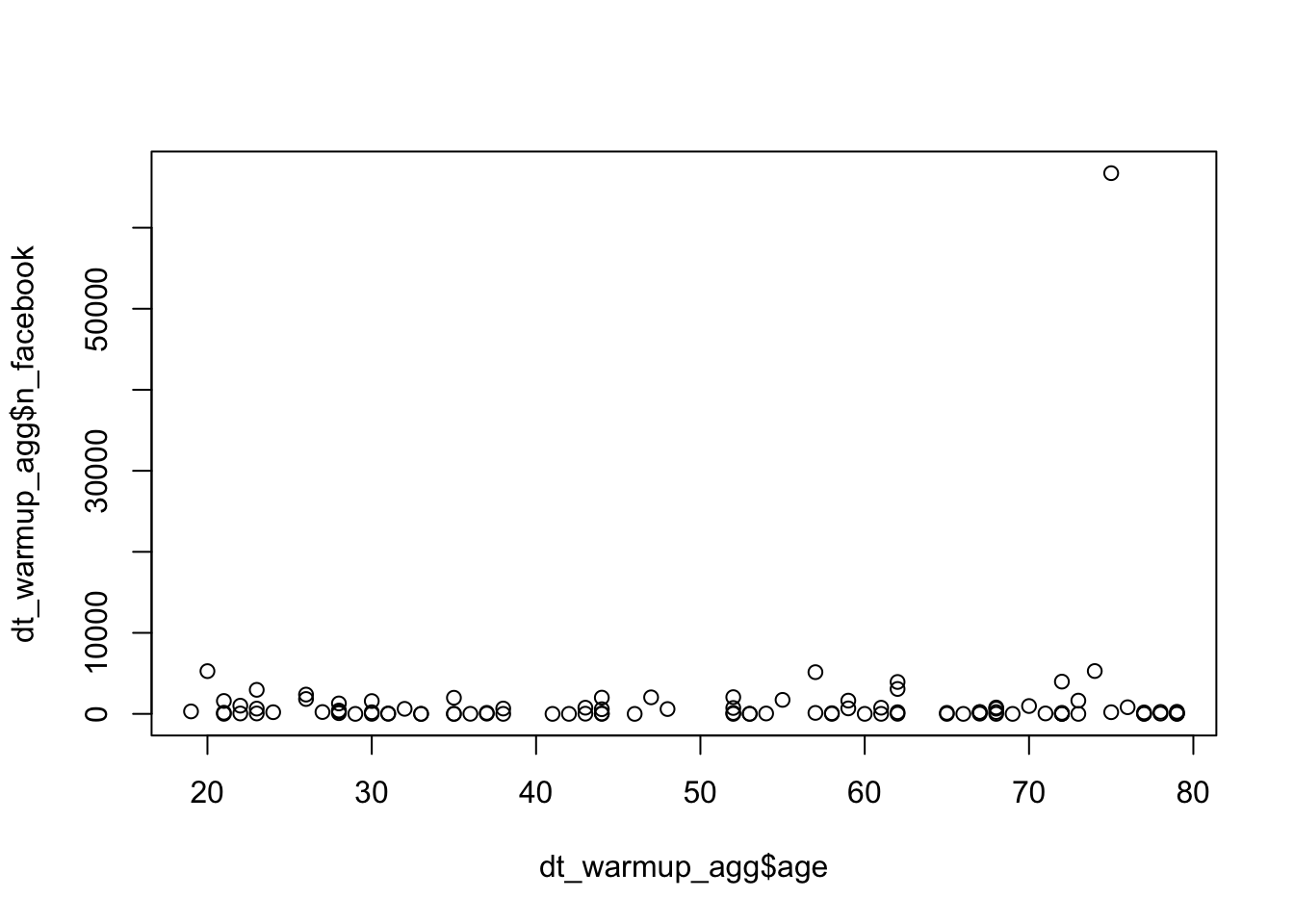
Pre-processing browsing data
Parsing URLs
Extracting hosts and domains
tidy R. As discussed in the paper’s SM A, the most flexible package to extract domains and hosts is adaR (Schoch and Chan 2023). Often, URLs in web browsing data miss the protocol (“https://”), in which case you need to add it before extracting domain or host. Let’s extract hosts and domains and print a random set of URLs along with extracted host and domain:
# add a protocol if necessary
dt <- dt %>%
  mutate(protocol = adaR::ada_get_protocol(url)) %>%
  mutate(url = ifelse(is.na(protocol), paste0("https://", url), url))

# extract the host
dt <- dt %>% mutate(host = adaR::ada_get_host(url))

# extract the domain
dt <- dt %>% mutate(domain = adaR::ada_get_domain(url))

# inspect some results
dt %>% select(url, host, domain) %>% sample_n(5)
url
1 https://www.google.com/search
2 https://www.mlb.com/tv/g566223/ve31e0f1a-986b-492a-afe7-614e8153b47f
3 https://www.lordandtaylor.com/shiseido-your-gift-with-any-75-shiseido-purchase-essential-energy-set/product/0500089152901
4 https://www.instagram.com/stories/lauriehernandez/
5 https://docs.google.com/document/d/1HjM902cuQdB1NEeg9BVFfplGP5amgln5cLiyQ5tlppY/edit
host domain
1 www.google.com google.com
2 www.mlb.com mlb.com
3 www.lordandtaylor.com lordandtaylor.com
4 www.instagram.com instagram.com
5 docs.google.com google.comwebtrackR The webtrackR package wraps functions by adaR and takes care of missing protocols:
# extract the host
wt <- extract_host(wt)

# extract the domain
wt <- extract_domain(wt)

# inspect some results
wt %>% select(url, host, domain) %>% sample_n(5)
url
1 https://opinionsresearch.com/survey/selfserve/58e/a25454
2 https://www.instagram.com/Roxxsaurus/
3 https://www.beasurveytaker.com/RouterSurvey/
4 https://www.net-research.com/e/425249/index.php
5 https://www.newegg.com/p/N82E16826814041
host domain
1 opinionsresearch.com opinionsresearch.com
2 www.instagram.com instagram.com
3 www.beasurveytaker.com beasurveytaker.com
4 www.net-research.com net-research.com
5 www.newegg.com newegg.comSQL. Presto SQL has an inbuilt function to extract the host:
SELECT *, URL_EXTRACT_HOST(url)) AS host
FROM dt
For domain extraction, it has no inbuilt function. One approach could be to upload the list of public suffixes as an SQL table, then to split up the URL host at every dot into parts; then to put the parts together incrementally, starting from the last part; finally match the resulting combinations to suffixes from the Public Suffix List. This strategy is explained in detail in this blog post. However, it is quite cumbersome, and the simpler approach is to download the list of unique hosts, extract the domains with the packages described above, and upload the table into the SQL database.
Extracting paths and queries
tidy R. Let’s extract paths and query and print a random set of URLs along with extracted paths and query:
# extract the path
dt <- dt %>% mutate(path = adaR::ada_get_pathname(url))

# extract the query
dt <- dt %>% mutate(query = adaR::ada_get_search(url))

# inspect some results
dt %>% select(url, path, query) %>% sample_n(5)
url
1 https://account.microsoft.com/rewards/
2 https://www.amazon.com/dp/1683370759
3 https://kelly--c.visualforce.com/apex/CandExpJobSearch
4 https://jezebel.com/prison-might-be-pretty-embarrassing-for-the-varsity-blu-1834442677
5 http://adserver.entertainow.com/promo/LHCwn3f9oCbAlnHY/
path query
1 /rewards/
2 /dp/1683370759
3 /apex/CandExpJobSearch
4 /prison-might-be-pretty-embarrassing-for-the-varsity-blu-1834442677
5 /promo/LHCwn3f9oCbAlnHY/ webtrackR. The package has a function for extracting the path, not yet one for extracting the query:
# extract the path
wt <- extract_path(wt)

# inspect some results
wt %>% select(url, path) %>% sample_n(5)
url
1 https://www.offroadexpo.com/video-scottsdale-off-road-expo-presented-by-nitto-2017
2 https://www.facebook.com/
3 https://www.instagram.com/candancesmith/
4 https://www.creditkarma.com/auth/logon
5 https://accounts.google.com/signin/v2/identifier
path
1 /video-scottsdale-off-road-expo-presented-by-nitto-2017
2 /
3 /candancesmith/
4 /auth/logon
5 /signin/v2/identifierAdditionally, webtrackR allows users to parse the path if it contains a human-readable string. As described in Section 4.3 of the paper, this information can be used for further classification. Since URL paths contain many non-human-readable strings, the package allows to specify whether to only keep strings consisting of letters, or only those consisting of English words:
# parse the paths into human-readable text
wt <- parse_path(wt, varname = "url", keep = "letters_only")

# inspect some results
wt %>% select(url, path, path_split) %>% sample_n(5)
url
1 https://docs.google.com/document/d/10zjeUc3kJmgr49lmjnbZYBwfcKQ83sYVaS8SN6twFpg/edit
2 https://mail.google.com/mail/u/0/
3 https://photos.google.com/search/May 25/photo/AF1QipMbW-Zj7WErhF4WVZP87Y0VrVFfrX3F-zQRSKT6
4 https://www.facebook.com/kentuckianahumor/photos/a.180682925896636/267987777166150/
5 https://www.google.com/search
path
1 /document/d/10zjeUc3kJmgr49lmjnbZYBwfcKQ83sYVaS8SN6twFpg/edit
2 /mail/u/0/
3 /search/May 25/photo/AF1QipMbW-Zj7WErhF4WVZP87Y0VrVFfrX3F-zQRSKT6
4 /kentuckianahumor/photos/a.180682925896636/267987777166150/
5 /search
path_split
1 document,d,edit
2 mail,u
3 search,photo
4 kentuckianahumor,photos,a
5 searchSQL. Presto SQL has inbuilt-functions to extract path and query:
SELECT *, URL_EXTRACT_PATH(url)) AS path, URL_EXTRACT_QUERY(url)) AS query
FROM dt
Defining visit duration
tidy R. The following code creates a timestamp-based duration variable, with a cutoff of 300 seconds and setting differences exceeding it to NA. Further, the visit before a device switch, as well as the last visit of a person, is set to NA.
# Define cutoff and replacement
cutoff <- 300
replacement <- NA

# create "next" timestamp and "next" device
dt <- dt %>%
  group_by(panelist_id) %>%
  mutate(timestamp_next = lead(timestamp, order_by = timestamp),
         device_next = lead(device, order_by = timestamp))

# create timestamp-based difference
dt <- dt %>%
  ungroup() %>%
  arrange(panelist_id, timestamp) %>%
  # compute raw time difference between timestamps
  mutate(timediff = timestamp_next - timestamp) %>%
  # set time difference to NA at device switch
  mutate(timediff = ifelse(device != device_next, NA, timediff)) %>%
  # set duration to time difference unless exceeding cutoff
  mutate(duration = ifelse(timediff > cutoff, NA, timediff)) %>%
select(-c(timestamp_next, device_next, timediff))webtrackR. The package wraps this logic in a function. It allows to set the cutoff value, the replacement value, and whether the duration before a device switch should be set to NA.
wt <- add_duration(
  wt, cutoff = 300, replace_by = NA,
device_switch_na = F, device_var = "device")SQL. In Presto SQL, the same can be done with the following:
SELECT panelist_id, wave, timestamp, url, device,
-- set duration to time difference unless exceeding cutoff, or before device switch
CASE
WHEN device != device_next THEN NULL
WHEN date_diff('second', timestamp, timestamp_next) > 300 THEN NULL
ELSE date_diff('second', timestamp, timestamp_next)
END AS duration
FROM
(SELECT *,
-- create "next" timestamp and "next" device
LEAD(timestamp) OVER(PARTITION BY panelist_id ORDER BY timestamp) AS timestamp_next,
LEAD(device) OVER(PARTITION BY panelist_id ORDER BY timestamp) AS device_next
FROM guide_testdata)
Defining referrals
tidy R. The below code examples implements the approach judged as optimal by Schmidt et al. (2023): A visit is defined as referred by a platform (e.g., Facebook) when it directly follows a visit to that platform and contains a certain pattern in its URL (e.g., “fbclid=”).
# the following assumes you have extracted the domain already
dt <- dt %>%
  # get previous domain
  group_by(panelist_id) %>%
  mutate(domain_previous = dplyr::lag(domain, order_by = timestamp)) %>%
  # flag referral
  mutate(referral = ifelse(domain_previous == "facebook.com" & grepl("fbclid=", url), 1, 0)) %>%
select(-c(domain_previous))webtrackR. The package implements the logic in a function that extracts the previous domain automatically and also allows getting referrals for multiple platforms/patterns:
wt <- add_referral(wt, platform_domains = "facebook.com", patterns = "fbclid=")SQL. The same approach would work as follows in Presto SQL, assuming the domain has been extracted:
SELECT *,
CASE
WHEN regexp_like('fbclid=', url) AND domain_previous = 'facebook.com' THEN 1
ELSE 0
END AS referral
FROM
(SELECT url, timestamp,
lag(domain) OVER (PARTITION BY panelist_id ORDER BY timestamp) AS domain_previous
FROM dt)
Filtering browsing data
Missing visits
R. For each participant, we can compute the proportion of the span of active days (i.e., the number of days between the first and last day of data for that person) out of the potential maximum of days (i.e., the difference between the first and last day of data collection). If this proportion is small, it could be an indication of missingness—of course, given certain theoretical assumptions. As the histogram below shows, there are indeed some subjects for which the proportion is small.
# define the maximum span of days as difference between first and last day
max_days <- as.numeric(max(as.Date(dt$timestamp)) - min(as.Date(dt$timestamp)))

# summarize per person
person_summary <- dt %>%
  mutate(date = as.Date(timestamp)) %>%
  group_by(panelist_id, date) %>%
  summarize(n_visits = n()) %>%
  group_by(panelist_id) %>%
  summarise(earliest = as.Date(min(date)),
            latest = as.Date(max(date))) %>%
  mutate(span_days = as.numeric(latest - earliest) + 1) %>%
  mutate(proportion = span_days / max_days)

# inspect the resulting proportion
hist(person_summary$proportion, breaks = 100)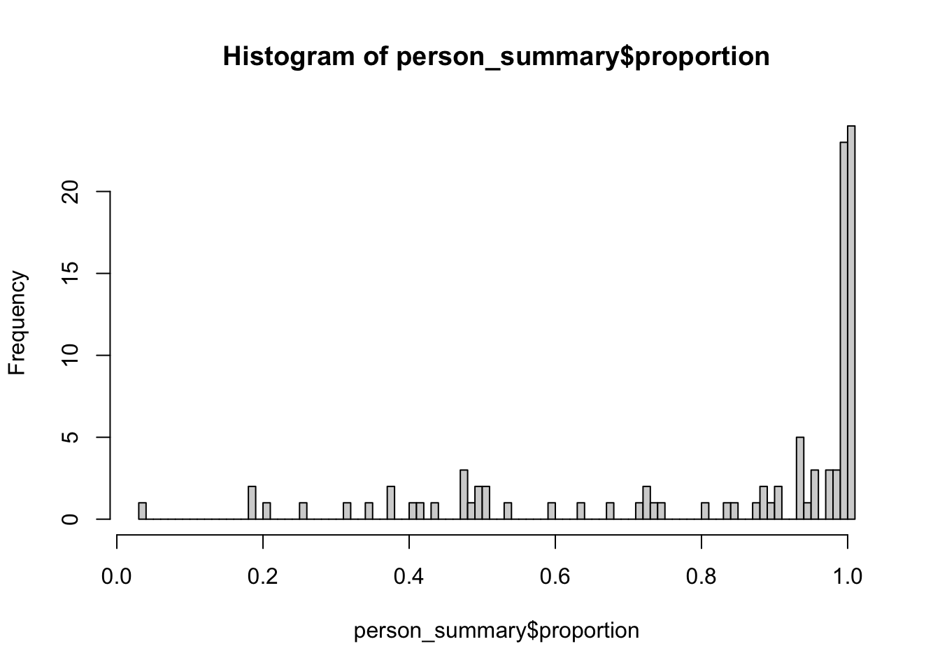
SQL. The same can be achieved in Presto as follows:
-- define the maximum span of days as difference between first and last day: 122
SELECT MAX(DATE(timestamp)) - MIN(DATE(timestamp))
FROM dt

-- summarize per person
SELECT panelist_id, earliest, latest,
DATE_DIFF('day', earliest, latest) AS span_days,
CAST(DATE_DIFF('day', earliest, latest) AS REAL) / max_days AS proportion
FROM
(SELECT panelist_id,
MIN(DATE(timestamp)) earliest, MAX(DATE(timestamp)) latest, 122 as max_days
FROM
(SELECT panelist_id, timestamp, COUNT() n_visits
FROM dt
WHERE wave = 1
GROUP BY panelist_id, timestamp)
GROUP BY panelist_id)
Duplicated visits
As we describe in the main paper, duplicates can be defined in several ways: as sequential visits to the same URL, after removing the URL’s fragment (Guess 2021); as visits to the same URL within the same day (Wojcieszak et al. 2022); or as sequential visits to the same URL that happen within one second. Alternatively, one can aggregate the duration of sequential visits to the same URL (Stier et al. 2022).
tidy R. The four methods can be applied to the data the following way:
# Guess 2021
dt <- dt %>%
  mutate(protocol = ada_get_protocol(url),
         host = ada_get_host(url),
         path = ada_get_pathname(url),
         query = ada_get_search(url),
         fragment = ada_get_hash(url))  %>%
  # construct URL without fragment
  mutate(url_without_fragment = paste0(protocol, host, path, query)) %>%
  select(-c(protocol, fragment)) %>%
  arrange(panelist_id, timestamp) %>%
  group_by(panelist_id) %>%
  # previous URL without fragment
  mutate(url_prev_without_fragment = lag(url_without_fragment, order_by = timestamp),
         person_visit_rank = 1:n()) %>%
  ungroup() %>%
  # if the previous URL is the same, then duplicate
  mutate(dupl_guess = ifelse(url_without_fragment == url_prev_without_fragment, 1, 0)) %>%
  # ... and the first visit of a person is 0, rather than NA
  mutate(dupl_guess = ifelse(person_visit_rank == 1, 0, dupl_guess)) %>%
  select(-c(url_prev_without_fragment, url_without_fragment))

# Wojcieszak et al 2022
dt <- dt %>%
  mutate(date = as.Date(timestamp)) %>%
  arrange(panelist_id, date, timestamp) %>%
  group_by(panelist_id, date, url) %>%
  # give unique number for URLs per date/person
  mutate(rep_number = 1:n()) %>%
  ungroup() %>%
  # any URL that has been visited already by person that day is duplicate
  mutate(dupl_wojc = ifelse(rep_number > 1, 1, 0)) %>%
  select(-c(date, rep_number))

# sequential visits to the same URL that happen within one second
cutoff <- 1
dt <- dt %>%
  arrange(panelist_id, timestamp) %>%
  group_by(panelist_id) %>%
  mutate(timestamp_prev = lag(timestamp, order_by = timestamp),
         url_prev = lag(url, order_by = timestamp),
         person_visit_rank = 1:n()) %>%
  ungroup() %>%
  mutate(created_diff = difftime(timestamp, timestamp_prev)) %>%
  # if previous URL is the same and within one sec, then duplicate
  mutate(dupl_onesec = ifelse((url == url_prev & created_diff <= cutoff), 1, 0)) %>%
  mutate(dupl_onesec = ifelse(person_visit_rank == 1, 0, dupl_onesec)) %>%
  select(-c(timestamp_prev, url_prev, person_visit_rank, created_diff))

# aggregate duration of sequential visits to the same URL
dt_agged <- dt %>%
  arrange(panelist_id, timestamp) %>%
  group_by(panelist_id) %>%
  mutate(url_group = cumsum(url != lag(url, def = first(url)))) %>%
  group_by(panelist_id, wave, url, url_group) %>%
  summarize(agg_duration = sum(duration, na.rm = T),
            timestamp_first = min(timestamp, na.rm = T)) %>%
  ungroup()

# inspect the resulting duplicate proportions
dt %>%
  summarize(prop_dupl_guess = sum(dupl_guess, na.rm = T) / n(),
            prop_dupl_wojc = sum(dupl_wojc, na.rm = T) / n(),
            prop_dupl_onesec = sum(dupl_onesec, na.rm = T) / n())
# A tibble: 1 × 3
prop_dupl_guess prop_dupl_wojc prop_dupl_onesec
<dbl> <dbl> <dbl>
1 0.395 0.662 0.139webtrackR. The package implements both the logic of treating sequential visits to the same URL that happen within one second as duplicates. It also allows users aggregation of consecutive visits to the same URL.
# flagging duplicates within one second
wt_dedup <- deduplicate(wt, method = "flag", within = 1)

# dropping duplicates within one second
wt_dedup <- deduplicate(wt, method = "drop", within = 1)

# aggregate duration of sequential visits to the same URL
wt_dedup <- deduplicate(wt, method = "aggregate", keep_nvisits = TRUE)SQL. Flagging/dropping duplicates defined as sequential visits within the same second, as well as aggregating the duration of sequential visits would work as follows in SQL:
-- flagging duplicates within one second
SELECT *,
CASE
WHEN timestamp_prev IS NULL THEN FALSE
WHEN date_diff('second', timestamp_prev, timestamp) <= 1 AND url = url_prev THEN TRUE
ELSE FALSE
END AS duplicate
FROM
(SELECT panelist_id,
timestamp, LAG(timestamp) OVER (PARTITION BY panelist_id ORDER BY timestamp) AS timestamp_prev,
url, LEAD(url) OVER (PARTITION BY panelist_id ORDER BY timestamp) AS url_prev
FROM dt)

-- dropping duplicates within one second
SELECT * FROM
(SELECT *,
CASE
WHEN timestamp_prev IS NULL THEN FALSE
WHEN date_diff('second', timestamp_prev, timestamp) <= 1 AND url = url_prev THEN TRUE
ELSE FALSE
END AS duplicate
FROM
(SELECT panelist_id,
timestamp, LAG(timestamp) OVER (PARTITION BY panelist_id ORDER BY timestamp) AS timestamp_prev,
url, LEAD(url) OVER (PARTITION BY panelist_id ORDER BY timestamp) AS url_prev
FROM dt))
WHERE duplicate = TRUE

-- aggregate duration of sequential visits to the same URL (assuming duration is extracted)
SELECT
sum(duration) AS agg_duration, MIN(timestamp) AS timestamp_first
FROM
(SELECT *,
SUM(new_url) OVER (PARTITION BY panelist_id ORDER BY timestamp) url_group
FROM
(SELECT *
CASE
WHEN url_no_query = LAG(url_no_query) OVER (PARTITION BY panelist_id ORDER BY timestamp) THEN 0
ELSE 1
END AS new_url
FROM dt
ORDER BY panelist_id, timestamp))
GROUP BY panelist_id, wave, url, url_group
Incentivized visits
R. To identify survey visits, you can use the list of hosts identified by Clemm von Hohenberg, Ventura, et al. (2024), which includes three types of entries: (1) hosts containing the word “survey”; (2) hosts matching the address of questionnaires platforms listed in a report by Bevec and Vehovar (2021); (3) those among the most frequented hosts identified as survey sites. Hence, this list is quite specific to the data analyzed in Clemm von Hohenberg, Ventura, et al. (2024). For example, in your data set that there may be other URL hosts containing the word “survey” not on our list. Thus, a more rigorous approach would be reproduce the approach on your own data set.
# download the list from OSF
filename <- "data/survey-click2earn-hosts.csv"
download.file(url = "https://osf.io/download/dw6cq/", destfile = filename)
survey_click2earn_hosts <- read.csv(filename)
rm(filename)

# match the list to the browsing data (assumes that host is already extracted)
dt <- dt %>%
  left_join(., survey_click2earn_hosts, by = c("host" = "url_host")) %>%
mutate(survey_flag = ifelse(!is.na(method), T, F))SQL. This would translate to Presto the following way, assuming the list of survey hosts is uploaded as a table:
-- join tracking data to list of survey hosts and flag visits
SELECT
d.url, d.url_host, s.method,
CASE
WHEN s.method IS NOT NULL THEN TRUE
ELSE FALSE
END AS survey_flag
FROM
(SELECT *, URL_EXTRACT_HOST(url) as url_host
FROM dat) d
LEFT JOIN survey_click2earn_hosts s ON d.url_host = s.url_host
Classifying browsing data
Many of the following operations require more coding flexibility, so we now proceed entirely in R.
Classifying by domains and hosts
R. To exemplify, we match the list of news sites by Wojcieszak et al. (2023) to the browsing data. Since not all of the news sites consist of a domain, but some also have a path (e.g., “yahoo.com/news”), we first need to split them up in two:
url <- "https://raw.githubusercontent.com/ercexpo/us-news-domains/main/us-news-domains-v2.0.0.csv"
news_list <- read.csv(url)

### Check which ones of our news sites are defined by domain only, which more than domain
news_list <- news_list %>%
  rename("domain_old" = domain) %>%
  mutate(https_domain = paste0("https://", domain_old)) %>%
  mutate(domain = adaR::ada_get_domain(https_domain)) %>%
  select(domain, domain_old) %>%
  mutate(domain_match = ifelse(domain == domain_old, T, F))

### News sites defined by domain
news_domains <- news_list %>%
  filter(domain_match == T) %>%
  select(domain) %>%
  mutate(news = 1) %>%
  filter(!duplicated(domain))

### News sites defined by more than domain (e.g. "yahoo.com/new")
### Change these to a string to be matched with regex
news_other <- news_list %>%
  filter(domain_match == F) %>%
  pull(domain_old) %>% paste(., collapse = "|")
Then, we match both the list of domains, and the list of domains with paths to the data:
dt <- dt %>%
  left_join(., news_domains, by = "domain") %>%
  mutate(news = ifelse(grepl(news_other, url), 1, news))
The logic is the same in webtrackR:
wt <- wt %>%
  left_join(., news_domains, by = "domain") %>%
  mutate(news = ifelse(grepl(news_other, url), 1, news))
Classifying by web site titles or paths
tidy R. The following R code lets you get titles for URLs with the help of the rvest package. Note that for a large number of URLs, this process can take a while. We therefore test the code with only a small selection of ten URLs. The results show that for a lot of cases, the title cannot be retrieved any more, which is unsurprising given the data collection happened in 2019.
# usually, you would get unique set of URls to speed up the process:
urls_unique <- data.frame(url = unique(dt$url))

# for now, we just get a random sample of ten:
urls_sample <- slice_sample(urls_unique, n = 10)

# for each URL, get the title (and set to NA if irretrievable)
urls_sample <- urls_sample %>%
  mutate(title = mapply(function(x) {
    return(
      tryCatch({
        print(x)
        html_text(html_node(read_html(x), "head title"))
      }, error = function(e) NA))}, url))
[1] "https://autismup.org/classes"
[1] "https://store.roosterteeth.com/products/rwby-ruby-sketch-t-shirt"
[1] "https://www.socialscour.com/ss3/search/web"
[1] "https://en.wikipedia.org/wiki/The_Perks_of_Being_a_Wallflower_(film)"
[1] "https://www.celebjihad.com/kelly-gale/kelly-gale-nude-and-sexy-photos-compilation"
[1] "https://worker.mturk.com/projects/3VKCYEEK5GMTPFGJS9C31OUU5FB1GV/tasks/3BAKUKE49HYJ95RMQEW5PANEBF0R19"
[1] "https://www.swagbucks.com/watch/video/309595317/it-helps-to-have-dads-advice-when-you-win-a-golden-globe-award"
[1] "https://www.amazon.com/gp/offer-listing/B009SNP2W6/SubscriptionId=AKIAJ7T5BOVUVRD2EFYQ&tag=camelproducts-20&linkCode=xm2&camp=2025&creative=165953&creativeASIN=B009SNP2W6"
[1] "https://old.reddit.com/r/TalesFromTheFrontDesk/comments/bhwubj/guest_was_angry_at_me_because_of_the_security/"
[1] "https://www.instagram.com/tidwell5451/channel/"# had we done this for all URLs, we could join back to data
# dt <- dt %>%
# left_join(., urls_unique, by = "url")
# inspect some results
urls_sample %>% head() url
1 https://autismup.org/classes
2 https://store.roosterteeth.com/products/rwby-ruby-sketch-t-shirt
3 https://www.socialscour.com/ss3/search/web
4 https://en.wikipedia.org/wiki/The_Perks_of_Being_a_Wallflower_(film)
5 https://www.celebjihad.com/kelly-gale/kelly-gale-nude-and-sexy-photos-compilation
6 https://worker.mturk.com/projects/3VKCYEEK5GMTPFGJS9C31OUU5FB1GV/tasks/3BAKUKE49HYJ95RMQEW5PANEBF0R19
title
1 <NA>
2 <NA>
3 <NA>
4 The Perks of Being a Wallflower (film) - Wikipedia
5 Kelly Gale Nude And Sexy Photos Compilation
6 Amazon Sign-InwebtrackR. The package wraps the above logic in a function and also allows to set the accepted language of the request. Note that this language setting does not overcome the fact that being in a different country will give you different results.
# get a random sample of ten rows:
wt_sample <- slice_sample(wt, n = 10)

# call the function
wt_sample <- add_title(wt_sample, lang = "en")

# inspect some results
wt_sample %>% select(url, title) %>% head()
Modeling browsing data
Browsing data can be modeled at many levels of analysis, e.g., the visit level or the participant-wave level. We start with the easiest case in which the data is aggregated on the participant level and joined to a survey.
tidy R. We summarize the number of all news visits and sum the duration of all news visits per person:
# aggregate number and duration of (news) visits
## this assumes you have joined the list of news sites to the data
## ... and that you have a duration variable
dt_person <- dt %>%
  mutate(news = ifelse(is.na(news), 0, news)) %>%
  group_by(panelist_id, news) %>%
  summarize(news_n = n(),
            news_sec = sum(duration, na.rm = T)) %>%
  pivot_wider(names_from = "news", values_from = c("news_n", "news_sec")) %>%
  mutate(across(c(news_n_1, news_sec_1), ~ ifelse(is.na(.), 0, .))) %>%
  ungroup() %>%
  mutate(total_n = news_n_1 + news_n_0, total_sec = news_sec_0 + news_sec_1) %>%
  select(panelist_id, total_n, total_sec, news_n = news_n_1, news_sec = news_sec_1)

dt_person <- dt_person %>%
left_join(., toy_survey, by = "panelist_id")webtrackR. The package has functions that allows you to derive the same summary:
# aggregate number of (news) visits
## this assumes you have joined the list of news sites to the data
wt_person_n <- sum_visits(wt, visit_class = "news")
wt_person_n <- wt_person_n[, c("panelist_id", "n_visits", "n_visits_news_1")]

# aggregate duration of (news) visits
## this assumes you have joined the list of news sites to the data
## ... and that you have a duration variable
wt_person_dur <- sum_durations(wt, visit_class = "news")
wt_person_dur <- wt_person_dur[, c("panelist_id", "duration_visits", "duration_visits_news_1")]
As webtrackR does not offer any functionality for modelling, we proceed with the dt_person object only.
Visits- vs time-based exposure
As we have summarized both duration and visits, we can do both visits-based and time-based modelling. For example, two regressions of political knowledge measured at the last wave (polknow_w4) on sociodemographics, total browsing and news exposure, once in terms of visits and once in terms of time would look like this:
# visits-based model
lm(polknow_w4 ~ age + sex + edu + news_n + total_n, data = dt_person) %>%
  summary()
Call:
lm(formula = polknow_w4 ~ age + sex + edu + news_n + total_n,
    data = dt_person)

Residuals:
     Min       1Q   Median       3Q      Max
-2.48150 -0.80613  0.02891  0.65293  2.34308

Coefficients:
              Estimate Std. Error t value Pr(>|t|)
(Intercept)  3.655e+00  3.536e-01  10.337  < 2e-16 ***
age          2.323e-03  5.501e-03   0.422  0.67382
sexmale     -2.615e-01  2.106e-01  -1.242  0.21748
edulow      -3.034e-01  2.735e-01  -1.109  0.27016
edumedium   -4.574e-01  2.442e-01  -1.873  0.06423 .
news_n      -2.560e-04  8.690e-05  -2.946  0.00407 **
total_n     -2.377e-05  5.571e-06  -4.266 4.78e-05 ***
---
Signif. codes:  0 '***' 0.001 '**' 0.01 '*' 0.05 '.' 0.1 ' ' 1

Residual standard error: 1.031 on 93 degrees of freedom
Multiple R-squared:  0.3258,    Adjusted R-squared:  0.2823
F-statistic: 7.491 on 6 and 93 DF,  p-value: 1.456e-06
# time-based model
lm(polknow_w4 ~ age + sex + edu + news_sec + total_sec, data = dt_person) %>%
summary()
Call:
lm(formula = polknow_w4 ~ age + sex + edu + news_sec + total_sec,
    data = dt_person)

Residuals:
     Min       1Q   Median       3Q      Max
-2.18260 -0.62362  0.04638  0.63464  2.27611

Coefficients:
              Estimate Std. Error t value Pr(>|t|)
(Intercept)  3.663e+00  3.390e-01  10.804  < 2e-16 ***
age          1.549e-03  5.293e-03   0.293   0.7705
sexmale     -2.644e-01  2.030e-01  -1.303   0.1959
edulow      -2.382e-01  2.618e-01  -0.910   0.3652
edumedium   -4.926e-01  2.340e-01  -2.105   0.0380 *
news_sec    -1.767e-05  4.057e-06  -4.356 3.41e-05 ***
total_sec   -5.232e-07  2.087e-07  -2.507   0.0139 *
---
Signif. codes:  0 '***' 0.001 '**' 0.01 '*' 0.05 '.' 0.1 ' ' 1

Residual standard error: 0.9931 on 93 degrees of freedom
Multiple R-squared:  0.375, Adjusted R-squared:  0.3347
F-statistic: 9.301 on 6 and 93 DF,  p-value: 5.591e-08
Accounting for skewness
If we think that the skew of the exposure variable needs to be accounted for by log-transformation, we could apply this transformation before running the model. Specifically, we take the natural log after adding 1 (so that a value of zero does not become undefined).
dt_person <- dt_person %>%
  mutate(across(c(news_n, total_n, news_sec, total_sec), ~ log(. + 1),
         .names = "{.col}_log"))
# log-transformed exposure (visits)
lm(polknow_w4 ~ age + sex + edu + news_n_log + total_n_log, data = dt_person) %>%
summary()
Call:
lm(formula = polknow_w4 ~ age + sex + edu + news_n_log + total_n_log,
    data = dt_person)

Residuals:
     Min       1Q   Median       3Q      Max
-1.85944 -0.56743  0.04893  0.48329  2.28713

Coefficients:
             Estimate Std. Error t value Pr(>|t|)
(Intercept)  5.077361   0.833504   6.092 2.50e-08 ***
age          0.001496   0.004290   0.349    0.728
sexmale     -0.166664   0.164114  -1.016    0.312
edulow      -0.081956   0.213298  -0.384    0.702
edumedium   -0.225455   0.191448  -1.178    0.242
news_n_log  -0.391735   0.054315  -7.212 1.44e-10 ***
total_n_log -0.048755   0.101509  -0.480    0.632
---
Signif. codes:  0 '***' 0.001 '**' 0.01 '*' 0.05 '.' 0.1 ' ' 1

Residual standard error: 0.8046 on 93 degrees of freedom
Multiple R-squared:  0.5897,    Adjusted R-squared:  0.5633
F-statistic: 22.28 on 6 and 93 DF,  p-value: 4.191e-16
# log-transformed exposure (duration)
lm(polknow_w4 ~ age + sex + edu + news_sec_log + total_sec_log, data = dt_person) %>%
summary()
Call:
lm(formula = polknow_w4 ~ age + sex + edu + news_sec_log + total_sec_log,
    data = dt_person)

Residuals:
     Min       1Q   Median       3Q      Max
-1.83086 -0.59240  0.03624  0.51253  2.33847

Coefficients:
                Estimate Std. Error t value Pr(>|t|)
(Intercept)    5.8064671  1.1611419   5.001 2.68e-06 ***
age            0.0009637  0.0044266   0.218    0.828
sexmale       -0.0606849  0.1695799  -0.358    0.721
edulow        -0.1268052  0.2174683  -0.583    0.561
edumedium     -0.2846867  0.1967174  -1.447    0.151
news_sec_log  -0.2799361  0.0418323  -6.692 1.64e-09 ***
total_sec_log -0.0614377  0.1062990  -0.578    0.565
---
Signif. codes:  0 '***' 0.001 '**' 0.01 '*' 0.05 '.' 0.1 ' ' 1

Residual standard error: 0.8284 on 93 degrees of freedom
Multiple R-squared:  0.5651,    Adjusted R-squared:  0.5371
F-statistic: 20.14 on 6 and 93 DF,  p-value: 5.808e-15
Controlling for overall browsing
Whether or not we need to control for overall browsing is a theoretical decision, and we can easily run the model with or without that control. Alternatively, we can also create a proportional measure of exposure:
dt_person <- dt_person %>%
  mutate(news_prop = news_n / total_n)
# no control for overall browsing
lm(polknow_w4 ~ age + sex + edu + news_n, data = dt_person) %>%
summary()
Call:
lm(formula = polknow_w4 ~ age + sex + edu + news_n, data = dt_person)

Residuals:
     Min       1Q   Median       3Q      Max
-2.63183 -0.81035 -0.01082  0.78559  2.79764

Coefficients:
              Estimate Std. Error t value Pr(>|t|)
(Intercept)  3.053e+00  3.526e-01   8.658  1.3e-13 ***
age          3.639e-03  5.974e-03   0.609 0.543932
sexmale     -2.005e-01  2.285e-01  -0.877 0.382472
edulow      -1.144e-01  2.935e-01  -0.390 0.697697
edumedium   -4.211e-01  2.655e-01  -1.586 0.116059
news_n      -3.637e-04  9.043e-05  -4.021 0.000117 ***
---
Signif. codes:  0 '***' 0.001 '**' 0.01 '*' 0.05 '.' 0.1 ' ' 1

Residual standard error: 1.122 on 94 degrees of freedom
Multiple R-squared:  0.1939,    Adjusted R-squared:  0.151
F-statistic: 4.522 on 5 and 94 DF,  p-value: 0.0009733
# control for overall browsing
lm(polknow_w4 ~ age + sex + edu + news_n + total_n, data = dt_person) %>%
summary()
Call:
lm(formula = polknow_w4 ~ age + sex + edu + news_n + total_n,
    data = dt_person)

Residuals:
     Min       1Q   Median       3Q      Max
-2.48150 -0.80613  0.02891  0.65293  2.34308

Coefficients:
              Estimate Std. Error t value Pr(>|t|)
(Intercept)  3.655e+00  3.536e-01  10.337  < 2e-16 ***
age          2.323e-03  5.501e-03   0.422  0.67382
sexmale     -2.615e-01  2.106e-01  -1.242  0.21748
edulow      -3.034e-01  2.735e-01  -1.109  0.27016
edumedium   -4.574e-01  2.442e-01  -1.873  0.06423 .
news_n      -2.560e-04  8.690e-05  -2.946  0.00407 **
total_n     -2.377e-05  5.571e-06  -4.266 4.78e-05 ***
---
Signif. codes:  0 '***' 0.001 '**' 0.01 '*' 0.05 '.' 0.1 ' ' 1

Residual standard error: 1.031 on 93 degrees of freedom
Multiple R-squared:  0.3258,    Adjusted R-squared:  0.2823
F-statistic: 7.491 on 6 and 93 DF,  p-value: 1.456e-06
# proportional measure
lm(polknow_w4 ~ age + sex + edu + news_prop, data = dt_person) %>%
summary()
Call:
lm(formula = polknow_w4 ~ age + sex + edu + news_prop, data = dt_person)

Residuals:
     Min       1Q   Median       3Q      Max
-3.12084 -0.80752  0.00932  0.84083  2.85510

Coefficients:
             Estimate Std. Error t value Pr(>|t|)
(Intercept)  2.952685   0.356308   8.287 7.96e-13 ***
age          0.004688   0.006059   0.774 0.440992
sexmale     -0.178137   0.231886  -0.768 0.444289
edulow      -0.045496   0.297556  -0.153 0.878806
edumedium   -0.382742   0.270193  -1.417 0.159920
news_prop   -8.331447   2.259622  -3.687 0.000379 ***
---
Signif. codes:  0 '***' 0.001 '**' 0.01 '*' 0.05 '.' 0.1 ' ' 1

Residual standard error: 1.135 on 94 degrees of freedom
Multiple R-squared:  0.1746,    Adjusted R-squared:  0.1307
F-statistic: 3.977 on 5 and 94 DF,  p-value: 0.002573
–>
References
Bevec, Domen, and Vasja Vehovar. 2021. “A WebSM Study: Web Survey Software 2021.” Faculty of Social Sciences, Centre for Social Informatics.
Clemm von Hohenberg, Bernhard, Sebastian Stier, Ana S Cardenal, Andrew Guess, Ericka Menchen-Trevino, and Magdalena Wojcieszak. 2024. “Analysis of Web Browsing Data: A Guide.”
Clemm von Hohenberg, Bernhard, Tiago Ventura, Magdalena Wojcieszak, Jonathan Nagler, and Joshua Tucker. 2024. “Survey Professionalism: New Evidence from Browsing Data.” 2024.
Guess, Andrew M. 2021. “(Almost) Everything in Moderation: New Evidence on Americans’ Online Media Diets.” American Journal of Political Science 65 (4): 1007–22. https://doi.org/10.1111/ajps.12589.
Schmidt, Felix, Frank Mangold, Sebastian Stier, and Roberto Ulloa. 2023. “Facebook as an Avenue to News: A Comparison and Validation of Approaches to Identify Facebook Referrals.” SocArXiv. 2023. osf.io/preprints/socarxiv/cks68.
Schoch, David, and Chung-hong Chan. 2023. “adaR: A Fast ’WHATWG’ Compliant URL Parser.” 2023. https://CRAN.R-project.org/package=adaR.
Schoch, David, Bernhard Clemm Von Hohenberg, Sebastian Stier, and Frank Mangold. 2023. “webtrackR: Analysing Web Tracking Data and Online News Behaviour.” 2023. https://CRAN.R-project.org/package=webtrackR.
Stier, Sebastian, Frank Mangold, Michael Scharkow, and Johannes Breuer. 2022. “Post Post-Broadcast Democracy? News Exposure in the Age of Online Intermediaries.” American Political Science Review 116: 768–74. https://doi.org/10.1017/S0003055421001222.
Wojcieszak, Magdalena, Bernhard Clemm von Hohenberg, Andreu Casas, Ericka Menchen-Trevino, Sjifra de Leeuw, Alexandre Gonçalves, and Miriam Boon. 2022. “Null Effects of News Exposure: A Test of the (Un) Desirable Effects of a ‘News Vacation’and ‘News Binging’.” Humanities and Social Sciences Communications 9 (1): 1–10.
Wojcieszak, Magdalena, Ericka Menchen-Trevino, Bernhard Clemm von Hohenberg, Sjifra de Leeuw, João Gonçalves, Sam Davidson, and Alexandre Gonçalves. 2023. “Non-News Websites Expose People to More Political Content Than News Websites: Evidence from Browsing Data in Three Countries.” Political Communication, 1–23.